Let's talk about the paper "Attention Is All You Need." The one that changed AI as we knew it.

It all starts with the Transformer architecture, which uses an Encoder-Decoder structure. But the real discovery is the thing that made everything click, the Attention Mechanism. So let's do what we did with embeddings. Start from first principles, bring in some maths, and actually understand how this thing works instead of just memorizing the diagram.

1. The Inputs (A Quick Recap)

Before we get into attention, a quick grounding. Every word gets converted into a vector through an embedding matrix, a big lookup table where each row is one word's vector representation. "Cat" has an index, you grab that row, you get a vector of real numbers. If any of that is new to you, the embeddings post walks through all of it from scratch, vocabulary, lookup, why integers aren't enough, the whole thing. It's better if you gave that a read first, before geting into this one, that's definitely necessarly.

For us, the important part is what comes after the embedding. Because here's the problem.

Take the sentence "The cat sat." After the embedding layer, we have three vectors:

Token	Embedding $h_t$
The	$[0.2,\;0.8,\;0.4,\;0.1]$
cat	$[0.9,\;0.3,\;0.2,\;0.7]$
sat	$[0.5,\;0.6,\;0.9,\;0.4]$

The three vectors are fine, but none of them know about each other. The embedding for "cat" has no idea that "sat" comes after it. The embedding for "sat" has no idea who performed the action. Three words, three vectors, three separate rooms. Nobody's communicating.

We need something that lets every word communicate with every other word. That something is self-attention.

2. The Core Mechanism: Self-Attention

The Self-Attention lives in this equation:

$$\text{Attention}(Q, K, V) = \text{Softmax}\!\left(\frac{QK^T}{\sqrt{d_k}}\right)V$$

We're going to build every piece of this from scratch. But keep it in the back of your mind. By the end, you'll be able to read it like a sentence.

The Big Idea

Three people in a meeting. Alice, Bob, Charlie.

Alice wants information. She asks everyone: "Who has something relevant to my question?" Everyone responds. Alice decides whose answer is most useful, then combines their answers weighting the useful ones more.

That's attention. Every token asks a question. Every other token responds. The token combines the useful responses, weighted by relevance.

Why Three Vectors?

Instead of using the embedding directly, the Transformer creates three new vectors from every embedding: Query (Q), Key (K), and Value (V).

These aren't three different words. They're three different representations of the same word. A person has a face, an ID card, and a personality. Same person. Different representation depending on what you need.

Starting Point

$d_{model} = 4$. Our word "cat" has embedding

$h = \begin{bmatrix} 0.9 & 0.3 & 0.2 & 0.7 \end{bmatrix}$

Row vector. Shape $1 \times 4$. This is our raw material.

Creating Q, K, and V

The paper writes $q = hW_Q$, $\;k = hW_K$, $\;v = hW_V$.

What Is $W_Q$?

Say $d_{model} = 4$ and $d_k = 3$. Then $W_Q$ is a $4 \times 3$ matrix.

$$W_Q = \begin{bmatrix} 0.5 & 0.2 & 0.8 \\ 0.1 & 0.9 & 0.3 \\ 0.7 & 0.4 & 0.2 \\ 0.6 & 0.5 & 0.1 \end{bmatrix}$$

These numbers are learned parameters. Initially random, then eventually optimized through gradient descent. Nobody picks them by hand.

The Multiplication

$h$ is $1 \times 4$. $W_Q$ is $4 \times 3$. Multiply them, you get $1 \times 3$.

$q = \begin{bmatrix} ? & ? & ? \end{bmatrix}$

First column: $0.9(0.5) + 0.3(0.1) + 0.2(0.7) + 0.7(0.6) = 0.45 + 0.03 + 0.14 + 0.42 = 1.04$. Repeat for every column. You get

$q = \begin{bmatrix} 1.04 & 0.83 & 0.93 \end{bmatrix}$

Same process for $W_K$ and $W_V$. Three multiplications. Three output vectors. Same input.

Why Three Different Matrices Though?

Imagine you're at a library. The books are on the shelves. Each book has a title on the spine and content inside. You walk up and ask: "Which books are about machine learning?"

Your question is the Query. The title on each book's spine is the Key. The actual pages are the Value.

Now notice, you compare your question against the titles. You don't rip open every book and read the pages to decide if it's relevant. Once the title matches, then you read the pages.

Query → compare with Keys → retrieve Values

This separation means the model decides where to look independently from what information to pull. Two different jobs, two different projections.

Why Not Just Use the Embedding Directly?

Because one embedding has to serve too many purposes. The word "bank" could mean a financial institution or the side of a river. A single vector mixes all of that together.

By learning separate $W_Q$, $W_K$, $W_V$, the model can emphasize different aspects of the same embedding depending on the role. The Query projection highlights what the token is looking for. The Key projection highlights features that help other tokens identify it. The Value projection shapes the information that actually gets passed along.

These projections are learned. The model figures out what's useful on its own.

A Thing People Get Wrong

A lot of people think: "First compute Q, then use Q to compute K, then use K to compute V." Nope. All three come directly from the same embedding, in parallel.

        h
        │
  ┌─────┼─────┐
  │     │     │
  WQ    WK    WV
  │     │     │
  ▼     ▼     ▼
  Q     K     V

The embedding branches into three parallel projections. No sequencing. No dependency between them.

Computing Attention Scores

Now we have Q and K for every token. And the model needs to answer a very specific question.

Take "The cat sat on the mat." We're processing the word "sat". The model asks: "Which words should I pay attention to in order to understand 'sat'?"

Maybe "cat" is very important who sat? Maybe "mat" is somewhat important where? And "The" is… not very important.

So we want a score for every word:

Word	Importance
The	0.1
cat	0.9
sat	0.6
on	0.3
mat	0.8

How do we get these numbers? Each word is a vector. We compare the Query of the current word against the Key of every other word. And the Transformer uses the dot product for that comparison.

The Dot Product

If $\mathbf{a} = [a_1, a_2, a_3, \ldots]$ and $\mathbf{b} = [b_1, b_2, b_3, \ldots]$, the dot product is the sum of the products of corresponding elements:

$\mathbf{a} \cdot \mathbf{b} = a_1 b_1 + a_2 b_2 + a_3 b_3 + \cdots$

One number comes out. A similarity score. Two vectors pointing in similar directions → big positive number. Perpendicular → zero. Opposite → negative.

Let's see it with actual vectors.

Example 1 — Similar Vectors

$\mathbf{v_1} = [3, 4]$, $\;\mathbf{v_2} = [2, 3]$

$\mathbf{v_1} \cdot \mathbf{v_2} = (3 \times 2) + (4 \times 3) = 6 + 12 = \boxed{18}$

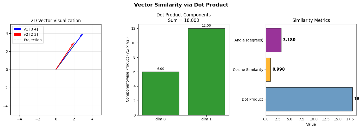
Cosine similarity $= \frac{18}{5.0 \times 3.606} \approx 0.998$. Angle $\approx 3.18°$. Nearly the same direction. Highly similar.

Example 2 — Perpendicular Vectors

$\mathbf{v_1} = [1, 0]$, $\;\mathbf{v_2} = [0, 1]$

$\mathbf{v_1} \cdot \mathbf{v_2} = (1 \times 0) + (0 \times 1) = 0$

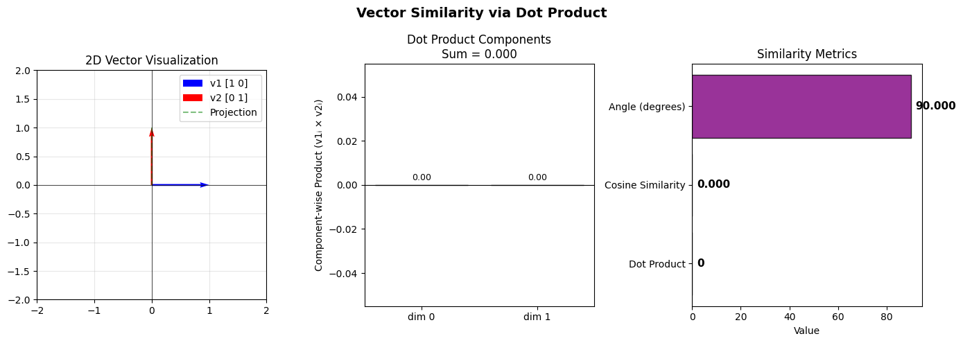
Cosine similarity $= 0$. Angle $= 90°$. Perpendicular. Completely unrelated.

Example 3 — Opposite Vectors

$\mathbf{v_1} = [2, 3]$, $\;\mathbf{v_2} = [-2, -3]$

$\mathbf{v_1} \cdot \mathbf{v_2} = (2 \times -2) + (3 \times -3) = -4 + (-9) = \boxed{-13}$

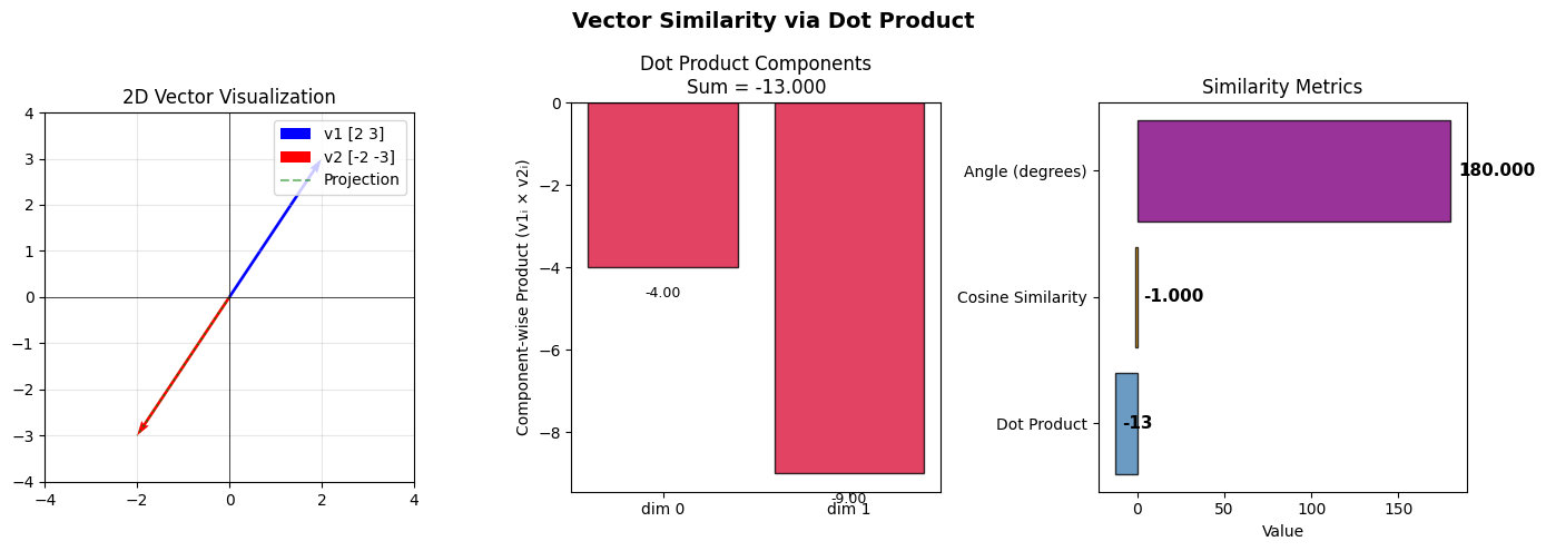
Cosine similarity $= -1$. Angle $= 180°$. Exactly opposite. Maximally dissimilar.

The dot product gives a raw score, but it's influenced by vector magnitude. Cosine similarity normalizes that by dividing by the magnitudes, giving a clean $-1$ to $1$ range. Same idea from the embeddings post. The Transformer uses the raw dot product for speed, but the intuition is identical.

Why Matrix Multiplication for $QK^T$?

Imagine a sentence of three words:

Word	Query	Key
The	$q_1$	$k_1$
cat	$q_2$	$k_2$
sat	$q_3$	$k_3$

We want to compare $q_2$ with every key. Score(cat, The). Score(cat, cat). Score(cat, sat). Then repeat for every query against all keys.

Instead of computing these one at a time, we can compute all of them simultaneously. That's where the matrix comes in.

Suppose

$$Q = \begin{bmatrix} 1 & 2 \\ 3 & 4 \\ 5 & 6 \end{bmatrix}, \quad K = \begin{bmatrix} 2 & 1 \\ 0 & 3 \\ 4 & 2 \end{bmatrix}$$

Each row of $Q$ is one query. Each row of $K$ is one key. Shape is $3 \times 2$ for both. Three words, two-dimensional keys.

According to linear algebra, we can't multiply $Q$ and $K$ directly — the inner dimensions don't match. $3 \times 2$ times $3 \times 2$ doesn't work. So we transpose $K$:

$$K^T = \begin{bmatrix} 2 & 0 & 4 \\ 1 & 3 & 2 \end{bmatrix}$$

Now $Q$ is $3 \times 2$ and $K^T$ is $2 \times 3$. Inner dimensions match. We get a $3 \times 3$ result.

Let's calculate step by step.

Row 1 of Q: $[1, 2]$

• Col 1: $(1 \cdot 2) + (2 \cdot 1) = 4$
• Col 2: $(1 \cdot 0) + (2 \cdot 3) = 6$
• Col 3: $(1 \cdot 4) + (2 \cdot 2) = 8$

Row 2 of Q: $[3, 4]$

• Col 1: $(3 \cdot 2) + (4 \cdot 1) = 10$
• Col 2: $(3 \cdot 0) + (4 \cdot 3) = 12$
• Col 3: $(3 \cdot 4) + (4 \cdot 2) = 20$

Row 3 of Q: $[5, 6]$

• Col 1: $(5 \cdot 2) + (6 \cdot 1) = 16$
• Col 2: $(5 \cdot 0) + (6 \cdot 3) = 18$
• Col 3: $(5 \cdot 4) + (6 \cdot 2) = 32$

$$QK^T = \begin{bmatrix} 4 & 6 & 8 \\ 10 & 12 & 20 \\ 16 & 18 & 32 \end{bmatrix}$$

What Does This Matrix Mean?

Each row corresponds to a Query. Each column corresponds to a Key.

	The	cat	sat
The	4	6	8
cat	10	12	20
sat	16	18	32

Row 2, Column 3 = 20 means: how much should "cat" attend to "sat"? Every token is compared with every other token in a single matrix multiplication. One operation. All pairwise scores. That's the elegance.

But look at those numbers. 4, 6, 8, 10, 12, 20, 16, 18, 32. They're raw scores. Unbounded. Some are large, some small. We can't use them directly as weights — they don't sum to 1, and they aren't probabilities. We need to fix that.

3. Softmax: Turning Scores Into Weights

Those raw dot-product scores could be anything. 4. 32. Negative numbers. Huge numbers. We need them to become weights. Numbers between 0 and 1 that sum to exactly 1, so we can use them as a weighted average.

That's what Softmax does.

For a vector of scores $[z_1, z_2, z_3]$, Softmax converts each one:

$$\text{Softmax}(z_i) = \frac{e^{z_i}}{\sum_j e^{z_j}}$$

Exponentiate each score. Divide by the sum of all exponentiated scores. The result: every value is between 0 and 1, and they all add up to 1.

Let's run it on row 2 of our score matrix, the row for "cat": $[10, 12, 20]$.

$$e^{10} \approx 22026, \quad e^{12} \approx 162755, \quad e^{20} \approx 485165196$$

Sum $\approx 485349977$.

$$\text{Softmax} = \left[\frac{22026}{485349977},\; \frac{162755}{485349977},\; \frac{485165196}{485349977}\right] \approx [0.00005,\; 0.0003,\; 0.9996]$$

Look at what happened. The score of 20 dominates. After Softmax, "cat" attends almost entirely to "sat" and basically ignores "The" and itself. The big score wins. The small scores get squashed toward zero.

That's the behavior we want. The model learns to make the relevant scores big and the irrelevant ones small, and Softmax turns that into a clean probability distribution.

Why Divide by $\sqrt{d_k}$?

One more detail in the equation, and it's easy to skip past, but it matters.

$$\text{Attention}(Q, K, V) = \text{Softmax}\!\left(\frac{QK^T}{\sqrt{d_k}}\right)V$$

That $\sqrt{d_k}$ in the denominator is scaling. The dot product of two vectors of dimension $d_k$ has a variance that grows with $d_k$. Bigger vectors → bigger dot products → bigger scores. And when scores get very large, Softmax saturates it, pushes almost all the weight onto one token and zeros out everything else. The gradients become tiny. Training stalls.

Dividing by $\sqrt{d_k}$ keeps the variance of the scores around 1, no matter how large $d_k$ is. Softmax stays in its sensitive range. The Gradients flow an the training works.

(It's a small fix. But the paper specifically calls it out, and without it, deep Transformers train poorly. One of those unglamorous engineering details that makes the whole thing function.)

Multiplying by $V$: The Actual Output

We have our attention weights. Softmax gave us $[0.00005,\; 0.0003,\; 0.9996]$ for the "cat" row. Now we use those weights to compute a weighted sum of the Value vectors.

Suppose the Value vectors for our three words are:

$$v_{\text{The}} = \begin{bmatrix} 0.1 & 0.5 & 0.3 \end{bmatrix}, \quad v_{\text{cat}} = \begin{bmatrix} 0.9 & 0.2 & 0.7 \end{bmatrix}, \quad v_{\text{sat}} = \begin{bmatrix} 0.4 & 0.8 & 0.6 \end{bmatrix}$$

The output for "cat" is:

$$\text{output}_{\text{cat}} = 0.00005 \cdot v_{\text{The}} + 0.0003 \cdot v_{\text{cat}} + 0.9996 \cdot v_{\text{sat}}$$ $$\approx 0.9996 \cdot \begin{bmatrix} 0.4 & 0.8 & 0.6 \end{bmatrix} \approx \begin{bmatrix} 0.4 & 0.8 & 0.6 \end{bmatrix}$$

The output is almost entirely the Value of "sat". Because the attention weights said "cat" should attend to "sat". The new representation of "cat" is now infused with information from "sat."

And that's the whole mechanism. Every token starts as its own embedding. After self-attention, every token becomes a blend of information from all tokens, weighted by relevance. The embedding for "cat" now knows about "sat". The embedding for "sat" now knows about "cat". They've talked to each other.

The equation, one more time:

$$\text{Attention}(Q, K, V) = \text{Softmax}\!\left(\frac{QK^T}{\sqrt{d_k}}\right)V$$

You can read it now. Project into Q, K, V. Compare Q with K via dot product. Scale. Softmax into weights. Weighted sum of V. That's attention.

4. Multi-Head Attention: Why One Head Isn't Enough

Here's a question:

In the sentence "The cat sat on the mat because it was tired," what does "it" refer to?

You know it's "cat". But the model has to figure that out. And "figure that out" isn't one single relationship. "It" needs to attend to "cat" for who. But maybe another part of the model also needs to attend to "mat" for where. And another part might track the grammar that "it" is singular, so the verb should be "was".

One attention head can only learn one pattern of relationships. One set of $W_Q$, $W_K$, $W_V$. One way of looking at the sentence.

So the Transformer uses multiple heads. Say 8, or 16, or 64. Each head gets its own $W_Q$, $W_K$, $W_V$. Each head learns a different relationship. One head tracks syntax. Another tracks coreference. Another tracks semantic roles. Another tracks positional patterns.

The process:

1. Split $d_{model}$ into $h$ smaller dimensions. If $d_{model} = 512$ and $h = 8$, each head works in a $64$-dimensional subspace.
2. Run attention independently in each head. Eight separate attention computations.
3. Concatenate all the outputs back together.
4. Project through one final linear layer $W_O$ to mix the information.

$$\text{MultiHead}(Q, K, V) = \text{Concat}(\text{head}_1, \ldots, \text{head}_h) \, W_O$$

where each $\text{head}_i = \text{Attention}(QW_i^Q, KW_i^K, VW_i^V)$.

The key insight: it's not more computation for the sake of more computation. It's letting the model look at the same sentence through multiple lenses simultaneously. One head can't do everything. Eight heads can each specialize.

(And here's a fun consequence: because each head operates on a smaller slice of the embedding, the total computation is roughly the same as one big attention. You get the benefit of multiple perspectives almost for free.)

5. Position: How the Model Knows Order

We've been talking about tokens as if they exist in a vacuum. But... they don't.

"The cat sat" and "sat cat The" have the same words but completely different meanings. The order matters here.

And here's the problem. Self-attention treats every token as a set, not a sequence. The dot product between "cat" and "sat" is the same regardless of which one comes first. Attention is permutation-invariant which shuffle the tokens, and the attention scores don't change.

So the Transformer needs to inject positional information before attention runs.

Positional Encoding

The original paper adds a fixed positional encoding to each embedding. For position $pos$ and dimension $i$:

$$PE_{(pos, 2i)} = \sin\!\left(\frac{pos}{10000^{2i/d_{model}}}\right)$$ $$PE_{(pos, 2i+1)} = \cos\!\left(\frac{pos}{10000^{2i/d_{model}}}\right)$$

Sine for even dimensions. Cosine for odd ones. Different frequencies for different dimensions.

You don't need to memorize the formula. The intuition is this: each position gets a unique "fingerprint" made of sine and cosine waves at different frequencies. Position 0 looks different from position 1, which looks different from position 2, and so on. And because sine and cosine are smooth, nearby positions have similar encodings. Position 5 is closer to position 6 than to position 50.

The embedding becomes:

$$\text{input to attention} = h_t + PE_t$$

Just add them. The word's meaning and its position get blended into one vector before self-attention ever sees it.

(Modern Transformers often use learned positional embeddings or rotary positional embeddings (RoPE) instead of fixed sine/cosine. The principle is the same: give the model a way to know where each token sits in the sequence. The implementation varies.)

6. The Encoder Block: Attention + Think + Normalize

Okay. We have multi-head self-attention. We have positional encoding. But the Transformer doesn't stop there. Attention lets tokens communicate. After that, each token needs to think about what it just learned.

That "thinking" step is a Feed-Forward Network.

The Feed-Forward Network

After attention, each token's representation is passed through a small neural network, a two linear layers with a non-linearity in between:

$$\text{FFN}(x) = W_2 \cdot \text{ReLU}(W_1 x + b_1) + b_2$$

The first layer projects the vector up to a larger dimension, typically $4 \times d_{model}$. ReLU introduces non-linearity. The second layer projects it back down to $d_{model}$.

Why? Attention mixes information between tokens. The FFN processes information within each token independently. It's the "okay, I've gathered context from everyone else, now let me actually reason about it" step.

Residual Connections and Layer Normalization

Two more ingredients left, they sound boring but they're not. Bear with it for now, I promise we're getting to the end.

Residual connections. After attention, the output is added back to the original input:

$$\text{output} = x + \text{Attention}(x)$$

Same after the FFN:

$$\text{output} = x + \text{FFN}(x)$$

Why? Cause Deep networks lose information as signals pass through many layers. The residual connection gives the gradient a shortcut, a highway straight back to earlier layers. Without it, deep Transformers can't train. The original paper stacks 6 encoder layers. Modern models stack 80, 96, 128. Residual connections are what make that depth possible.

Layer Normalization. After each sub-layer, the activations are normalized: mean shifted to 0, variance scaled to 1. Keeps the numbers from exploding or vanishing as they pass through dozens of layers.

So one full encoder layer looks like this:

Input
  │
  ├──→ Multi-Head Self-Attention ──→ Add (residual) ──→ Layer Norm
  │                                                         │
  ├──→ Feed-Forward Network ────────→ Add (residual) ──→ Layer Norm
  │                                                         │
  └─────────────────────────────────────────────────────────→ Output

And the Encoder isn't one of these. It's a stack. The original paper uses $N = 6$ identical layers. Each layer refines the representation further. Layer 1 captures basic relationships. Layer 3 captures more complex ones. Layer 6 captures high-level semantic structure.

7. The Decoder: Generating One Word at a Time

Everything we've built so far is the Encoder. It reads the entire input at once and produces a rich, context-aware representation. But if the task is generation translation, summarization, writing then we need to produce output one token at a time.

That's the Decoder.

Masked Self-Attention

The Decoder has self-attention too, but with a twist. When generating the 5th word, the model should not be able to see the 6th, 7th, or 8th words. They don't exist yet. It can only look at what's already been generated.

So we apply a mask. In the $QK^T$ score matrix, every position that corresponds to a future token is set to $-\infty$ before Softmax. And $e^{-\infty} = 0$. So those positions get zero attention weight. The model literally cannot attend to the future.

Score matrix (before mask):      After mask:
[ 4   6   8 ]                   [ 4   6   8  ]
[ 10  12  20 ]                  [ 10  12  20 ]
[ 16  18  32 ]                  [ -∞  -∞  32 ]

Row 3 can only see itself. Row 2 can see itself and row 1. Row 1 can only see itself. Causal. Left-to-right. Exactly how you generate text.

Cross-Attention

The Decoder has a second attention layer, and this one is different. In self-attention, Q, K, and V all come from the same sequence. In cross-attention, the Query comes from the Decoder, but the Keys and Values come from the Encoder's output.

$$\text{CrossAttention}(Q_{\text{dec}}, K_{\text{enc}}, V_{\text{enc}})$$

This is how the Decoder "reads" the input. If we're translating "The cat sat" into French, the Decoder is generating "Le chat s'est assis" one word at a time. When it's generating "chat", it sends a Query that says "what word in the source am I translating right now?" The Keys and Values from the Encoder respond, and the attention weights point back to "cat" in the English sentence.

The Decoder looks at the Encoder's understanding of the input to decide what to generate next.

The Full Decoder Layer

One Decoder layer has three sub-layers:

1. Masked self-attention the generated tokens talk to each other, but can't peek ahead.
2. Cross-attention the generated tokens attend to the Encoder's output.
3. Feed-forward network independent processing per token.

Each sub-layer has its own residual connection and layer normalization. Same pattern as the Encoder. And again, the paper stacks $N = 6$ of these layers.

8. The Output: From Vectors to Words

The Decoder produces a vector for each generated position. But we don't want vectors. We want words.

The final step is a linear projection from $d_{model}$ back to the vocabulary size $V$, followed by a Softmax:

$$\text{logits} = h_{\text{final}} \cdot W_{\text{vocab}}$$ $$\text{probabilities} = \text{Softmax}(\text{logits})$$

This gives a probability distribution over every word in the vocabulary. The model picks the next token, maybe the highest-probability word, maybe sampled with some randomness for creativity and appends it to the sequence. Then it runs the Decoder again with the new, longer sequence. And again. And again. Until it generates an end-of-sequence token.

One word at a time. Each word conditioned on all previous words. That's autoregressive generation.

The Finale: Putting It All Together

Let's take a breath and zoom out for a bit

Input tokens
    │
    ▼
Embedding + Positional Encoding
    │
    ▼
┌──────────────────────────┐
│  ENCODER (× N layers)    │
│  ├ Self-Attention        │
│  ├ Add & Layer Norm      │
│  ├ Feed-Forward          │
│  └ Add & Layer Norm      │
└──────────┬───────────────┘
           │
           │  (Encoder output: K, V for cross-attention)
           ▼
┌──────────────────────────┐
│  DECODER (× N layers)    │
│  ├ Masked Self-Attention │
│  ├ Add & Layer Norm      │
│  ├ Cross-Attention ◄─────┼── from Encoder
│  ├ Add & Layer Norm      │
│  ├ Feed-Forward          │
│  └ Add & Layer Norm      │
└──────────┬───────────────┘
           │
           ▼
Linear + Softmax → next token probability
           │
           ▼
      Output tokens

Input goes in. Embeddings get positions. The Encoder builds a deep, contextual understanding through six layers of attention and feed-forward processing. The Decoder generates output one token at a time, using masked self-attention to respect order, cross-attention to reference the input, and feed-forward layers to reason. The final projection turns vectors back into words.

And the whole thing is trained end-to-end with backpropagation. Every $W_Q$, $W_K$, $W_V$, every FFN weight, every layer norm parameter, all learned from data. Nobody hand-wired any of it.

And That how Tranformer shaped the current evolution in AI. I hope you had a great time and understood how transformer works now